LiDAR (Light Detection and Ranging) or point cloud data is useful when we are conducting high-resolution spatial analysis such as viewshed/viewscape, watershed runoff, and other analysis based on digital surface/terrain models. But collecting LiDAR data may challenge for data download and storage because the data is huge even for a median-scale area like a city. Converting a large amount of point cloud into a raster for spatial analysis could be even more computationally expensive. To facilitate data search and downloading, I wrote a simple R packge - dsmSearch, which is basically a wrapped API using R as an interface. I have introduced a little about this package in one of my previous tutorial. The package can help search and download LiDAR data sourced from USGS (United States Geological Survey) But I think that post was definitely not enough to make the large-scale data collection easier. Overall, the package itself does not computationally address the challenge of the large-scale data collection. There is a trick we can use to play with this package to make the large-scale data collection process more efficient.

The trick introduced in this tutorial may be usable in the case that one has a large number of geo-located samples across a large-scale area and does not need an entire piece of terrain data. Basically, it is based on the concept of grid search. A large-scale study area can be sliced into a set of subarea, which can stabilize the downloading process and make the further data analysis and conversion easier. I use the city of Detroit, MI as an example to demonstrate the idea.

1 Create grids given a focus area

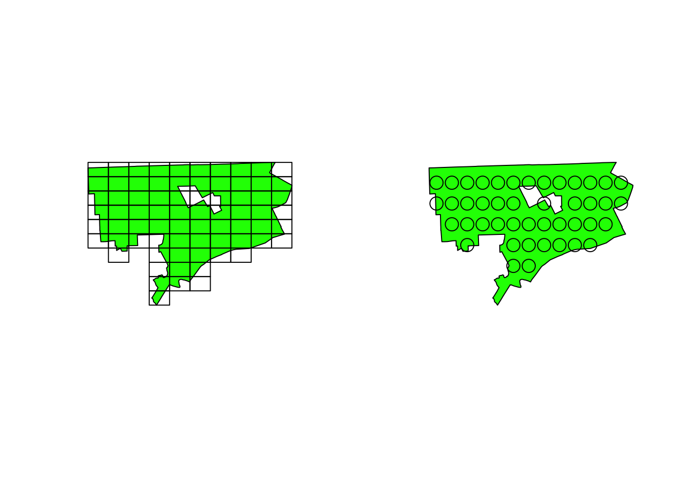
There are two ways to generated a set of grids: bounding box and point samples.

First, I got a bbox of Detroit and randomly samples 50 points with the bbox.

# set up grids on the bbox
# download the shapefile of Detroit and create a bbox
poly <- tigris::places('MI', progress_bar=FALSE)
d_poly <- poly[poly$NAME=='Detroit',]
d_grid <- sf::st_make_grid(
  d_poly,
  n=c(10,10),
  crs = sf::st_crs(d_poly)
)
# only keep those grids overlapping with the bondary of Detroit
grid_binary <- sf::st_intersects(d_grid, d_poly)
grid_binary <- as.data.frame(grid_binary)[,1]
d_grid <- d_grid[grid_binary]

# set up grids by sampled locations
# create 50 samples
samples <- sf::st_sample(d_poly, size = 50, type = 'regular')

# use each point as a center point to create a set of grids
library(tidyr)
sample_grids <- lapply(samples, function(pt) {
  coor <- sf::st_coordinates(pt)
  p <- as.data.frame(coor) %>% 
    sf::st_as_sf(coords=c('X', 'Y'), crs = 4326) %>%
    sf::st_transform(2253)
  # set a buffer with 3280ft (1km)
  buffer <- sf::st_buffer(p, 3280)
  buffer <- sf::st_transform(buffer, 4326)
  # grid <- sf::st_make_grid(
  #   buffer,
  #   n=c(1,1),
  #   crs = sf::st_crs(buffer)
  # )
  # return(grid[[1]])
})
sample_grids <- do.call(rbind, sample_grids)
sample_grids <- sf::st_as_sf(sample_grids)

2 Download LiDAR data grid by grid

The function get_lidar can download data and store it in the memory if the directory for saving is not specified. However, for the large-scale data collection, the total size of data may be run out of the memory capacity, crashing the process. Therefore, I recommend to specify a directory to download the data to a hard drive. Once the data collection is done, we can convert each LiDAR file into raster or extract other information for further data analysis.

for(each in d_grid) {
  bbox <- sf::st_bbox(each)
  # convert the crs if it is not degree (optinal)
  bbox <- bbox %>% sf::st_transform(4326)
  data <- dsmSearch::get_lidar(bbox=bbox, 
                               folder='path/to/save/file')
}

for(each in sample_grids) {
  bbox <- sf::st_bbox(each)
  # convert the crs if it is not degree (optinal)
  bbox <- bbox %>% sf::st_transform(4326)
  data <- dsmSearch::get_lidar(bbox=bbox, 
                               folder='path/to/save/file')
}