1 Introduction
Babo tea - “波霸奶茶” in Chinese (also known as pearl milk tea or bubble milk tea) - with its origins in Taiwan, holds particular appeal among customers interested in Asian cuisines and cultural experiences. Enjoying boba tea while waiting for a table at a restaurant or as a delightful treat after dining is a widespread practice in urban areas like Los Angeles, CA. Boba-tea shops and restaurants often serve as complementary businesses. Customers who visit a restaurant for a meal might seek a boba-tea shop nearby for a refreshing beverage afterward, or vice versa. This symbiotic relationship enhances the overall dining and leisure experience for customers, encouraging a culture of “meal followed by a treat.” By strategically positioning these establishments near one another, business owners can capitalize on cross-promotion opportunities and drive increased foot traffic.
2 Research Question and Methods
Questions:
The study aims to understand this symbiotic relationship by investigating the linkage between operating conditions and the spatial connection between boba-tea shops and restaurants within urban areas, specifically focusing on how their proximity influences business opportunities in Monterey Park and Alhambra, California.
The study answered two questions:
- If boba-tea shops are more likely located within the 10-minute walking distance of restaurants?
- How are the degree and edge weight of spatial network between boba-tea shops and restaurants associated with their operating conditions within the 10-minute walking distance between them?
Method:
To understand the complementary businesses between boba-tea shops and restaurants based on spatial analysis, the point of interest (POI) sourced from Yelp API was utilized to conduct spatial data analysis. I assumed the greater rate and more review count of a boba-tea shop or a restaurant may indicate better operating conditions.
For data collection, a grid-based approach was adopted to systematically search for POIs of boba-tea shop and restaurant within the study area. In this data acquisition, the id, coordinates, rate, and review count fields of POI data were extracted for data analysis.
The analysis phase involved linear regression and network analysis methods to investigate the relationship between operating conditions (rate and review) and network metrics (degree and edge weight), and identify patterns of spatial connectivity within the network.
3 Data Acquisition
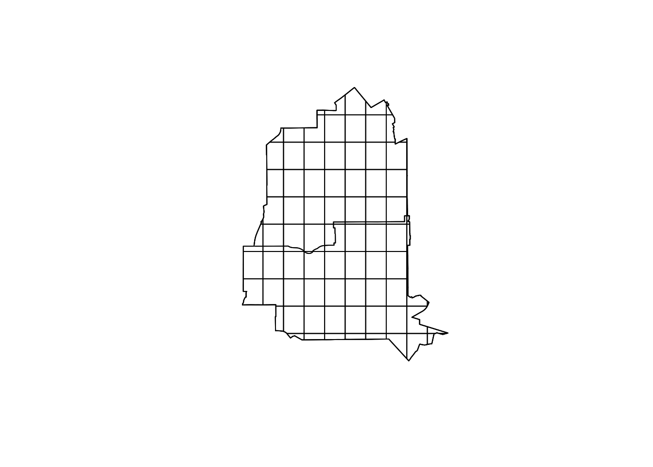
Polygons of city boundary of Montery Park and Alhambra were downloaded from the US Census and merged for creating search girds.
A set of grids was created based on the bounding box of the study area. Within each grid, bthe oba tea shop and restaurant POIs were collected using the centroid and diagonal line of the grid as the location and radius, with “boba tea” and “restaurants” as key words. As a result, 539 restaurants and 112 boba-tea shops were collected.
##                       id              name         x        y rate review
## 1 jtg1AqCL6Fl6NDmAyAz6cw XOXO Sushi Lounge -118.1516 34.03311  4.0      9
## 2 diw55Vr3EeEO6g81IN84ng          Teriroll -118.1533 34.03248  4.6    238
## 3 8mUug5Vtd84W_y-Uo-lVhw          Soul Mex -118.1526 34.03301  5.0      2
## 4 3bU_sFDzaK21eE7gxuhOmA    Tacos La Guera -118.1526 34.03325  2.8     31
## 5 ilUxHLaYrS3HLmfYHMOf4A           The Hat -118.1464 34.03721  3.8    872
## 6 Olxl-pkozXb1BphIu9K5qQ        Everytable -118.1458 34.03716  4.3     36
##                       id                             name         x        y
## 1 sCFtWUo96yaE2JRaRyQ-oA   It's Boba Time - Monterey Park -118.1459 34.03761
## 2 z2qfXr92DeA9Fx-1PPp-tQ                 Bumblebee Donuts -118.1261 34.03183
## 3 kV1rxJN8JaDlllmpmd9v_Q Little Dimples Playground & Cafe -118.0953 34.03359
## 4 aZEUq76ipghkDDy4DLGO3A                        Pokitomik -118.0934 34.03364
## 5 7SzKYGpwdzVpaDj53qCXug                         Boba Ave -118.1434 34.04025
## 6 RuJxN6KXiKAUTXt6Pk7f4Q              Mister Fried Potato -118.1425 34.03908
##   rate review
## 1  3.8    226
## 2  4.5    173
## 3  4.3    209
## 4  4.1    105
## 5  4.1    758
## 6  4.4    123
4 Data Analysis and Interpretation
###Edge Document Creation: The first step involves generating an “edge” document to represent potential customer pathways between restaurants and boba tea shops. This is achieved using the expand.grid function, which creates all possible combinations of restaurant and boba tea shop IDs. These combinations symbolize hypothetical connections or routes customers might take from a restaurant to a boba tea shop and vice versa.
Augmenting Edge Document:
The edge document is then enriched with the ratings (rate) and the number of reviews (review) for both restaurants and boba tea shops. This is done by joining the edge document with subsets of the restaurant and boba tea shop data frames, respectively. The resulting edge document contains comprehensive information about each potential pathway, including identifiers for the establishments and metrics indicating their operating conditions: popularity and customer satisfaction.
Node Document Creation:
Subsequently, a “node” document is created by merging the data frames of restaurants and boba tea shops into a single dataset. A new attribute, type, is introduced to distinguish between the two kinds of establishments within the unified dataset. This classification facilitates further analysis and visualization by providing a straightforward way to differentiate between restaurants and boba tea shops.
Spatial Transformation:
The node dataset undergoes a transformation to a spatial format (sf object) to enable geographic analysis and mapping. Each node, representing either a boba tea shop or a restaurant, is assigned spatial coordinates (x, y). These coordinates are then transformed to a specific spatial reference system (SRS) for consistency and accuracy in spatial operations.
Edge Geometry and Weight Assignment:
The connections between nodes are spatialized through the creation of edge geometries, converting abstract connections into spatial lines. The lengths of these lines, representing walking distances, are calculated and used to assign weights to each edge. Edges exceeding 800 m (beyond a 10-minute walking distance) are excluded from the dataset. In addition, Min-max normalization was employed to rescale the weights with the range from 0 to 1.
Node Degree and Weight Metrics:
For each node, the degree (the number of connections it has with other nodes) is computed. This metric provides insight into the node’s centrality within the network. Additionally, the average and minimum weights (distances) of the edges connected to each node are calculated. These metrics help in understanding the accessibility of each establishment and the spatial distribution of boba tea shops and restaurants relative to each other.
## Simple feature collection with 6 features and 8 fields
## Geometry type: POINT
## Dimension:     XY
## Bounding box:  xmin: 1985847 ymin: 559077.3 xmax: 1986537 ymax: 559600.8
## Projected CRS: NAD83(2011) / California zone 5
## # A tibble: 6 × 9
##   id                     name         rate review type  degree min_wght men_wght
##   <chr>                  <chr>       <dbl>  <int> <chr>  <dbl>    <dbl>    <dbl>
## 1 jtg1AqCL6Fl6NDmAyAz6cw XOXO Sushi…   4        9 rest…      1   0.907     0.907
## 2 diw55Vr3EeEO6g81IN84ng Teriroll      4.6    238 rest…      0   0         0
## 3 8mUug5Vtd84W_y-Uo-lVhw Soul Mex      5        2 rest…      0   0         0
## 4 3bU_sFDzaK21eE7gxuhOmA Tacos La G…   2.8     31 rest…      1   0.980     0.980
## 5 ilUxHLaYrS3HLmfYHMOf4A The Hat       3.8    872 rest…      6   0.0834    0.440
## 6 Olxl-pkozXb1BphIu9K5qQ Everytable    4.3     36 rest…      6   0.0638    0.399
## # ℹ 1 more variable: geometry <POINT [m]>
## Simple feature collection with 6 features and 9 fields
## Geometry type: LINESTRING
## Dimension:     XY
## Bounding box:  xmin: 1985910 ymin: 559146.7 xmax: 1986537 ymax: 559644.5
## Projected CRS: NAD83(2011) / California zone 5
## # A tibble: 6 × 10
##   restrnt           shop  rt_rstr rvw_rst rat_shp rvw_shp distanc weight ln_wdth
##   <chr>             <chr>   <dbl>   <int>   <dbl>   <int>   <dbl>  <dbl>   <dbl>
## 1 jtg1AqCL6Fl6NDmA… sCFt…     4         9     3.8     226   726.  0.907      0.5
## 2 3bU_sFDzaK21eE7g… sCFt…     2.8      31     3.8     226   783.  0.980      0.5
## 3 ilUxHLaYrS3HLmfY… sCFt…     3.8     872     3.8     226    66.7 0.0834     0.1
## 4 Olxl-pkozXb1BphI… sCFt…     4.3      36     3.8     226    51.0 0.0638     0.1
## 5 hIr3N0KkWjlfEHmk… sCFt…     3.3     184     3.8     226    30.1 0.0376     0.1
## 6 tDpUrrY3Pco-sdJG… sCFt…     3.2     159     3.8     226    86.0 0.108      0.1
## # ℹ 1 more variable: geometry <LINESTRING [m]>
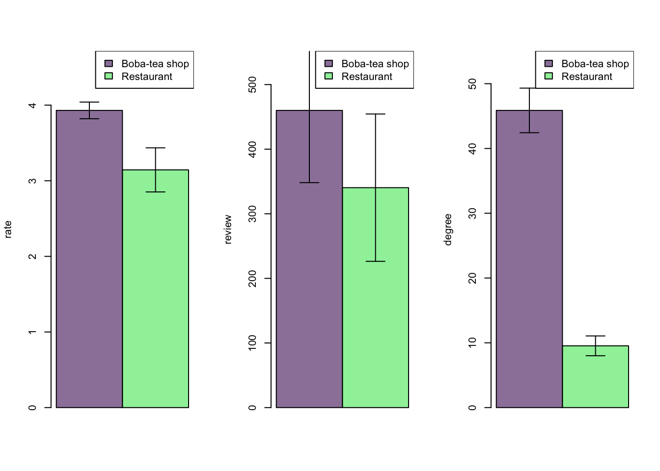
Descriptive analysis:
the mean values of ‘rate’, ‘degree’, and ‘review’ of boba-tea shops and restaurants were compared using a bar chart plot.
- Both boba tea shops and restaurants generally have good ratings, with boba tea shops showing slightly higher average ratings than restaurants.
- Boba tea shops have a significantly higher average number of reviews compared to restaurants, suggesting that boba-tea shops may receive more traffic or may have been established for longer periods, thus accumulating more reviews over time.
- The number of connections to each other in a network, is higher on average for boba-tea shops than restaurants, indicating that boba-tea shops may located within the intersected accessible areas of several restaurant.
Regression analysis:
Regression analysis was conducted to investigate the impact of the establishment’s network degree andaverage/minimum walking distance (min_weight and mean_weight) on its rating and number of reviews. Two linear regression models are specified:
- Model 1 examines the relationship between the number of reviews (review) and the explanatory variables (degree, min_weight, and mean_weight). This model aims to understand how these factors associate the number of reviews. The model suggests that the minimum and average walking distances significantly associate with the number of reviews for boba tea shops and restaurants, with the degree of network connectivity showing a non-significant effect. The minimum distance is positively associated with review number, whereas the average distance is negatively associated with review number. However, the overall explanatory power of the model is quite low, indicating that other unmeasured factors may be influencing customer reviews.
##
## Call:
## lm(formula = review ~ degree + min_wght + men_wght, data = nodeSpatial)
##
## Residuals:
##    Min     1Q Median     3Q    Max
## -570.6 -309.6 -178.6   54.5 4277.7
##
## Coefficients:
##             Estimate Std. Error t value Pr(>|t|)
## (Intercept)  199.280     56.091   3.553 0.000409 ***
## degree         2.077      1.579   1.316 0.188790
## min_wght    -422.908    156.180  -2.708 0.006951 **
## men_wght     442.598    155.643   2.844 0.004600 **
## ---
## Signif. codes:  0 '***' 0.001 '**' 0.01 '*' 0.05 '.' 0.1 ' ' 1
##
## Residual standard error: 573.2 on 647 degrees of freedom
## Multiple R-squared:  0.0316,	Adjusted R-squared:  0.02711
## F-statistic: 7.037 on 3 and 647 DF,  p-value: 0.0001164
- Model 2 explores how the same set of explanatory variables associates the customer rating (rate). This model indicates that the degree of network connectivity significantly and positively associate with the ratings of boba tea shops and restaurants, with minimal and non-significant impacts from minimum and average walking distances. However, as with the previous model on reviews, the overall explanatory power of the model is low, suggesting that other factors not included in this model might play a significant role in determining ratings.
##
## Call:
## lm(formula = rate ~ degree + min_wght + men_wght, data = nodeSpatial)
##
## Residuals:
##     Min      1Q  Median      3Q     Max
## -3.4019 -0.4033  0.4157  0.9239  2.0030
##
## Coefficients:
##              Estimate Std. Error t value Pr(>|t|)
## (Intercept)  3.076100   0.135242  22.745  < 2e-16 ***
## degree       0.015422   0.003806   4.052  5.7e-05 ***
## min_wght    -0.098349   0.376564  -0.261    0.794
## men_wght    -0.055938   0.375271  -0.149    0.882
## ---
## Signif. codes:  0 '***' 0.001 '**' 0.01 '*' 0.05 '.' 0.1 ' ' 1
##
## Residual standard error: 1.382 on 647 degrees of freedom
## Multiple R-squared:  0.03729,	Adjusted R-squared:  0.03283
## F-statistic: 8.355 on 3 and 647 DF,  p-value: 1.863e-05
5 Data Visualization and Interpretation
First, the road data was downloaded from OSM to be served as the map’s background. The road lines are transformed to match the coordinate reference system (CRS) of the study area. They are also clipped to ensure they only cover the study area. Maps displaying the spatial network of boba-tea shops and restaurants were constructed, visualizing attributes (e.g., degree, review, rate).
Map 1
For the map as below, a boba-tea shop may serve customers from multiple nearby restaurant (Fig 1). This implies that boba-tea shops are pivotal nodes, facilitating a broader network of connections within their accessible vicinity than restaurants do with neighboring boba-tea establishments.
Map 2
Most boba-tea shops are located in the area, where they can connect more restaurants with more review counts (Fig 2). The map can be a strategic asset, highlighting potential areas for establishing new business to tap into existing popularity and foot traffic patterns. It may also assist current business owners in understanding their positioning within the local market based on consumer feedback volumes.
Map 3
Both highly-rated and lower-rated businesses are scattered throughout the area, without a clear pattern of ratings clustering (Fig 3). For boba-tea shops and restaurants, factors other than location play a significant role in promoting their business.
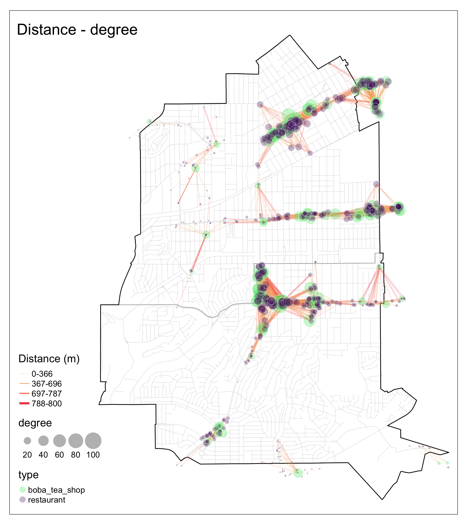 Figure 1
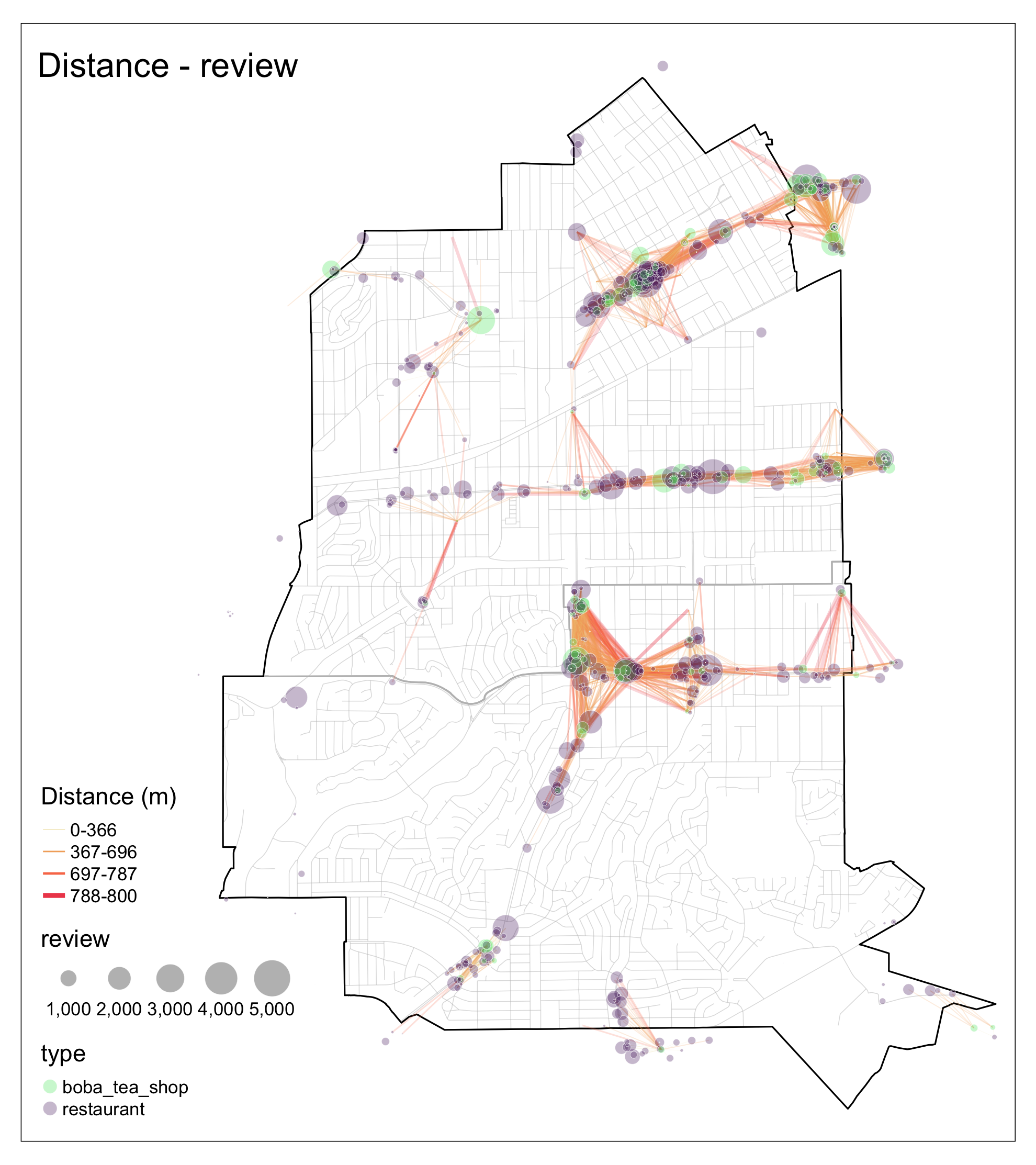 Figure 2
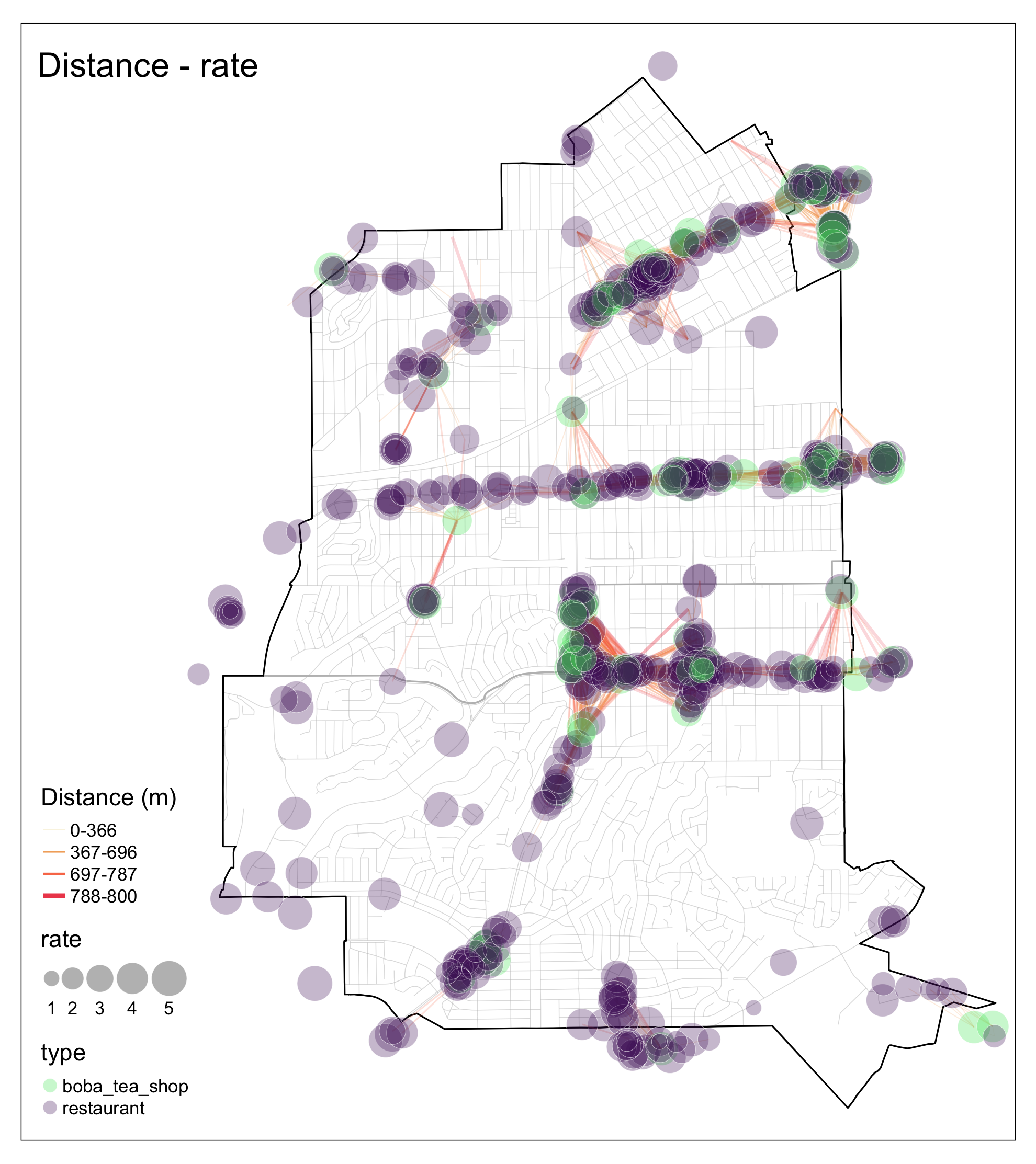 Figure 3
Code
# ------------------Study Area and Search Grid------------------------

# download the boundary of Monterey Park and Alhambra
place_poly <- tigris::places('CA')
MP_poly <- place_poly[place_poly$NAME=='Monterey Park',]
A_poly <- place_poly[place_poly$NAME=='Alhambra',]
place_poly <- sf::st_union(rbind(MP_poly, A_poly))
# create grids for searching Yelp POIs
place_grid <- sf::st_make_grid(
  place_poly,
  n=c(10,10),
  crs = sf::st_crs(place_poly)
)
place_grid <- sf::st_intersection(place_grid, place_poly)

#------------------collect poi data------------------------

# set up api key and url
API_key <- readr::read_file('api.txt')
url <- "https://api.yelp.com/v3/businesses/search"

# scratch babo tea store POIs via Yelp api
get_poi <- function(grid, url, API_key, keyword) {
  # get bbox of this grid
  bbox <- sf::st_bbox(grid)
  xmin <- bbox[1]
  ymin <- bbox[2]
  xmax <- bbox[3]
  ymax <- bbox[4]
  # make two diagonal points
  pt1 <- sf::st_sfc(sf::st_point(c(xmin, ymin)))
  pt1 <- pt1 %>% sf::st_set_crs(4326) %>%
    sf::st_transform(6423)
  pt2 <- sf::st_sfc(sf::st_point(c(xmax, ymax)))
  pt2 <- pt2 %>% sf::st_set_crs(4326) %>%
    sf::st_transform(6423)
  # calculate the center of the bbox
  center_x <- (xmin + xmax) / 2
  center_y <- (ymin + ymax) / 2
  # Calculate the radius to cover the bbox area
  # for searching data
  radius <- sf::st_distance(pt1, pt2) / 2
  # request POIs
  response <- httr::GET(
    url,
    httr::add_headers(Authorization = paste("Bearer", API_key)),
    query = list(
      term = keyword,
      latitude = center_y,
      longitude = center_x,
      radius = as.integer(radius),
      sort_by = "best_match",
      limit = 50
    )
  )
  results <- httr::content(response, "parsed")
  pois <- lapply(results$businesses, function(poi) {
    list(id = poi$id,
         name = poi$name,
         x = poi$coordinates$longitude,
         y = poi$coordinates$latitude,
         rate = poi$rating,
         review = poi$review_count)
  })
  pois_df <- do.call(rbind.data.frame, pois)
  return(pois_df)
}

df_list <- list()
for (i in 1:length(place_grid)) {
  df <- get_poi(place_grid[[i]], url, API_key, "boba tea")
  if (nrow(df) > 0) {
    df_list[[length(df_list)+1]] <- df
  }
}
boba_shops <- do.call(rbind.data.frame,df_list)
# remove duplicated rows
boba_shops <- unique(boba_shops)

# scratch restaurant POIs
df_list <- list()
for (i in 1:length(place_grid)) {
  df <- get_poi(place_grid[[i]], url, API_key, "restaurant")
  if (nrow(df) > 0) {
    df_list[[length(df_list)+1]] <- df
  }
}
restaurant <- do.call(rbind.data.frame,df_list)
# remove duplicated rows
restaurant <- unique(restaurant)
restaurant <- dplyr::anti_join(restaurant, boba_shops)

#------------------prepare data for data analysis and visualization------------------------

# create edge document, connecting restaurants to babo-tea shops
edge <- expand.grid(restaurant$id,
                    boba_shops$id)
names(edge) <- c('restaurant', 'shop')
# also add the rate of boba-tea shops and restaurants to the edge document
edge <- dplyr::left_join(
  edge,
  restaurant[,c('id', 'rate', 'review')],
  dplyr::join_by(restaurant == id)
)
edge <- dplyr::left_join(
  edge,
  boba_shops[,c('id', 'rate', 'review')],
  dplyr::join_by(shop == id)
)
names(edge) <- c("restaurant", "shop",
                 "rate.restaurant", "review.restaurant",
                 "rate.shop", "review.shop")

# combine the boba-tea shop and restaurant data frames as node document
node <- rbind(restaurant, boba_shops)
node$type <- ''
node['type'] <- unlist(lapply(node[,'id'], function(x){
  if (x %in% restaurant$id) {
    return('restaurant')
  } else {
    return('boba_tea_shop')
  }
}))

# create sf objects for spatial visualization
nodeSpatial <- node %>%
  sf::st_as_sf(coords=c("x", "y"), crs = 4326) %>%
  sf::st_transform(6423)
# create edge geometry and add wights based on length
edge2line <- stplanr::od2line(edge, nodeSpatial)
edge2line <- edge2line %>%
  dplyr::mutate(distance = as.numeric(sf::st_length(geometry)))
# drop the edges with length longer than 10-minute walk distance (800m)
edge2line <- subset(edge2line, distance <= 800)
# redefine edge by removing long connections
edge <- dplyr::inner_join(edge[,c(1,2)], edge2line[,c(1,2)])[,c(1,2)]
# normalize the weight
edge2line$weight <- unlist(lapply(edge2line$distance, function(x){
  (x - min(edge2line$distance))/(max(edge2line$distance) - min(edge2line$distance))
}))

brks <- quantile(edge2line$weight, probs=c(0, 0.5, 0.9, 0.99, 1))
edge2line <- edge2line %>% dplyr::mutate(
  line_width = dplyr::case_when(
    weight >= brks[1] & weight <= brks[2] ~ 0.1,
    weight > brks[2] & weight <= brks[3] ~ 0.3,
    weight > brks[3] & weight <= brks[4] ~ 0.5,
    weight > brks[4] & weight <= brks[5] ~ 1
  )
)
# create degree column for each node
g <- igraph::graph_from_data_frame(
  edge,
  directed = FALSE,
  vertices=nodeSpatial[,c('id', 'geometry')]
)
nodeSpatial$degree <- igraph::degree(g)

# calculate average and minimum walking distance for each node
nodeSpatial$mean_weight <- unlist(
  lapply(nodeSpatial$id, function(x){
    if (x %in% restaurant$id) {
      sub_edge <- subset(edge2line, restaurant == x)
    } else {
      sub_edge <- subset(edge2line, shop == x)
    }
    out <- mean(sub_edge$weight)
    if (is.na(out)) {
      out <- 0
    }
    return(out)
  })
)

nodeSpatial$min_weight <- unlist(
  lapply(nodeSpatial$id, function(x){
    if (x %in% restaurant$id) {
      sub_edge <- subset(edge2line, restaurant == x)
    } else {
      sub_edge <- subset(edge2line, shop == x)
    }
    out <- min(sub_edge$weight)
    if (is.infinite(out)) {
      out <- 0
    }
    return(out)
  })
)

#------------------data analysis------------------------

plot_data <- function(data, info) {
  if (info == 'rate') {
    bilan <- aggregate(rate~type , data=data , mean)
    stdev <- aggregate(rate~type , data=data , sd)
  } else if (info == 'degree') {
    bilan <- aggregate(degree~type , data=data , mean)
    stdev <- aggregate(degree~type , data=data , sd)
  } else if (info == 'review') {
    bilan <- aggregate(review~type , data=data , mean)
    stdev <- aggregate(review~type , data=data , sd)
  }
  rownames(bilan) <- bilan[,1]
  bilan <- as.matrix(bilan[,-1])
  # Plot boundaries
  lim <- 1.2*max(bilan)
  # A function to add arrows on the chart
  error.bar <- function(x, y, upper, lower=upper, length=0.1,...){
    arrows(x,y+upper, x, y-lower, angle=90, code=3, length=length, ...)
  }
  # calculate the standard deviation for each specie and condition:
  rownames(stdev) <- stdev[,1]
  stdev <- as.matrix(stdev[,-1]) * 1.96 / 10
  # add the error bar on the plot using my "error bar" function
  out_barplot <- barplot(bilan, beside=T, legend.text=T,
                         col=c(rgb(0.3,0.1,0.4,0.6),
                               rgb(0.3,0.9,0.4,0.6)),
                         ylim=c(0,lim), ylab=info)
  error.bar(out_barplot, bilan, stdev)
  legend("topright", legend=c("Boba-tea shop", "Restaurant"),
         fill=c(rgb(0.3,0.1,0.4,0.6), rgb(0.3,0.9,0.4,0.6)))
}

par(mfrow = c(1, 3))
# mean of rate of restaurants and shops
plot_data(nodeSpatial, 'rate')
# mean  of node degree of restaurants and shops
plot_data(nodeSpatial, 'review')
# mean of node degree of restaurants and shops
plot_data(nodeSpatial, 'degree')

# analyze the relationship between rate and degree and distance
model1 <- lm(review ~ degree + min_weight + mean_weight,
             data=nodeSpatial)

model2 <- lm(rate ~ degree + min_weight + mean_weight,
             data=nodeSpatial)

summary(model1)
summary(model2)

#------------------data visualization------------------------

# download road from OSM for map background
query <- osmdata::opq(bbox = sf::st_bbox(place_poly),
                      timeout = 20000) %>%
  osmdata::add_osm_feature(
    key = "highway",
    value = c('primary',
              'secondary',
              'tertiary',
              'unclassified',
              'residential')
  )
osm_data <- try({
  osmdata::osmdata_sf(query)
}, silent = TRUE)
road_lines <- osm_data$osm_lines$geometry
# clip
road_lines <- sf::st_transform(road_lines,
                               sf::st_crs(place_poly))
road_lines <- sf::st_intersection(road_lines,
                                  place_poly)

# spatial network
const_map <- function(show) {
  map <-
    tmap::tm_shape(road_lines) +
    tmap::tm_lines(col = 'grey', alpha=0.5, lwd=0.5) +
    tmap::tm_shape(A_poly) +
    tmap::tm_polygons(alpha=0, border.col = 'grey') +
    tmap::tm_shape(MP_poly) +
    tmap::tm_polygons(alpha=0, border.col = 'grey') +
    tmap::tm_shape(place_poly) +
    tmap::tm_polygons(alpha=0, border.col = 'black') +
    tmap::tm_shape(dplyr::arrange(edge2line, dplyr::desc(weight))) +
    tmap::tm_lines(
      #arguments that define the styles for color
      col="weight", alpha=0.2,
      breaks = brks,
      style="fixed", n = 4,
      palette=c('#ecda9a', '#f3ad6a', '#f97b57', '#ee4d5a'),
      legend.col.show = FALSE,
      #arguments that define the styles for line width
      lwd='line_width', scale=2,
      legend.lwd.show = FALSE
    ) +
    tmap::tm_add_legend(
      type=c('line'),
      col=c('#ecda9a', '#f3ad6a', '#f97b57', '#ee4d5a'),
      lwd=c(0.1, 0.3, 0.5, 1)*3,
      labels=c('0-366','367-696','697-787','788-800'),
      title='Distance (m)') +
    tmap::tm_shape(nodeSpatial) +
    tmap::tm_symbols(size=show,
                     scale=1.5,
                     col='type',
                     palette=c(rgb(0.3,0.9,0.4,0.6), rgb(0.3,0.1,0.4,0.6)),
                     alpha=0.3,
                     border.col='white',
                     border.alpha = 1,
                     border.lwd = 0.2,
                     shapes.legend.fill='gray',
                     title.size=c(show)) +
    tmap::tm_layout(legend.position = c('left', 'bottom'),
                    inner.margins = c(0.1,0.2,0.05,0.05),
                    title = paste0('Distance - ', show))
}
# make maps
map_degree <- const_map('degree')
map_review <- const_map('review')
map_rate <- const_map('rate')
# plot maps
tmap::tmap_mode('plot')
map_degree
map_review
map_rate